Bathymetry from multispectral aerial images via Convolutional Neural Networks

Dauer der Arbeit: 4 Monate
Abschluss: March 2020
Betreuer: Dr.-Ing. Gottfried Mandlburger, M.Sc. Michael Kölle
Prüfer: Prof. Dr.-Ing. Uwe Sörgel

Recently, optical approaches were applied more often to derive the depth of waterbodies. In shallow areas, the depth can be deduced mainly by modeling the signal attenuation in different bands. In this approach, it is examined how well a Convolutional Neural Network is able to estimate water depths from multispectral aerial images. To train on the actually observed slanted water distances, the net is trained with the original images rather than the orthophoto. The trained CNN is showing a standard deviation of 3 to 4 decimeters. It is able to recognize trends for varying depths and ground covers. Problems mainly occurred when facing sunglint or shaded areas.

Motivation

Reconstructing the surface of the earth by means of photogrammetry is an established method. Coordinates of object points can be computed via forward intersection when the respective point  is observed in two or more images. However, applying this procedure to water surfaces is more complex. Nevertheless, charting water depths is necessary, especially in shallow water areas for example when considering safe routing of ships, or when determining the volume of a lake which is needed for extinguishing fires. The complexity involves measuring of identical points due to the specular and dynamic nature of the water surface. Furthermore, there is refraction on the water surface because of transition of the image ray between two media. For generating an orthophoto this particularly means that every pixel in each image has its unique refracted ray corresponding  to the water surface which also may show local dynamics. Thus, to find the corresponding ground points of each pixel, this ray has to be traced from the respective image position, with its direction given by the orientation of the image, also considering the refraction on the water surface. Another point is that even if the direction of each ray is known, enough identical points have to be detected to calculate their coordinates with help of the intersecting rays from the images. That is also demanding, because the submerged ground is often homogeneous and in addition there is attenuation in the water. Also, because of reflection and other factors the same points can appear differently when taken from different perspectives.

Because of different magnitudes of absorption of light for various spectral bands in the water column, it is also possible to fit a linear or higher dimensional regression model to band ratios, approximating the relation from radiometry to depth. But as soon as the scene contains different types of vegetation on the ground of the water basin, a more complex regression model is needed. Furthermore, spectrally based bathymetry estimation is commonly carried out based on orthophotos. Not only are orthophotos of waters prone to geometric errors due to neglection of ray refraction at the water surface, but most also ignore the fact that only pixel values from the image center (nadir direction) directly relate to water depth whereas pixels from the edge of an image rather show the slanted water distance. Each pixel of an aerial image, in turn, stores radiometric information which is mainly related to the potentially slanted under water distance of the respective image ray. Especially for aerial images taken with wide-angle lenses it is therefore beneficial to perform the bathymetry estimation based on the (oriented) images rather than the orthophoto.

To extend the linear regression approach, a Convolutional Neural Network (CNN) can be used to cope with variations in bottom reflectance. Pixel-wise depth estimation based on the oriented aerial images require the slanted water distance for the image pixels for training. This information can

e.g. be derived from bathymetric LiDAR (Light Detection And Ranging), especially when carried out concurrently with the image capture. The CNN based approach has the advantage that spatial context information is taken into account. The reliability of the net is therefore increased, since proximity often implies similar depths.

In this thesis, the approach of training a convolutional network to predict the slanted distances from image rays inside a waterbody, will be examined. Next to quality assessment and critical discussion, it will also be discussed to which extent the Coastal Blue channel has an influence on the network.

Multi View Stereo

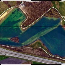
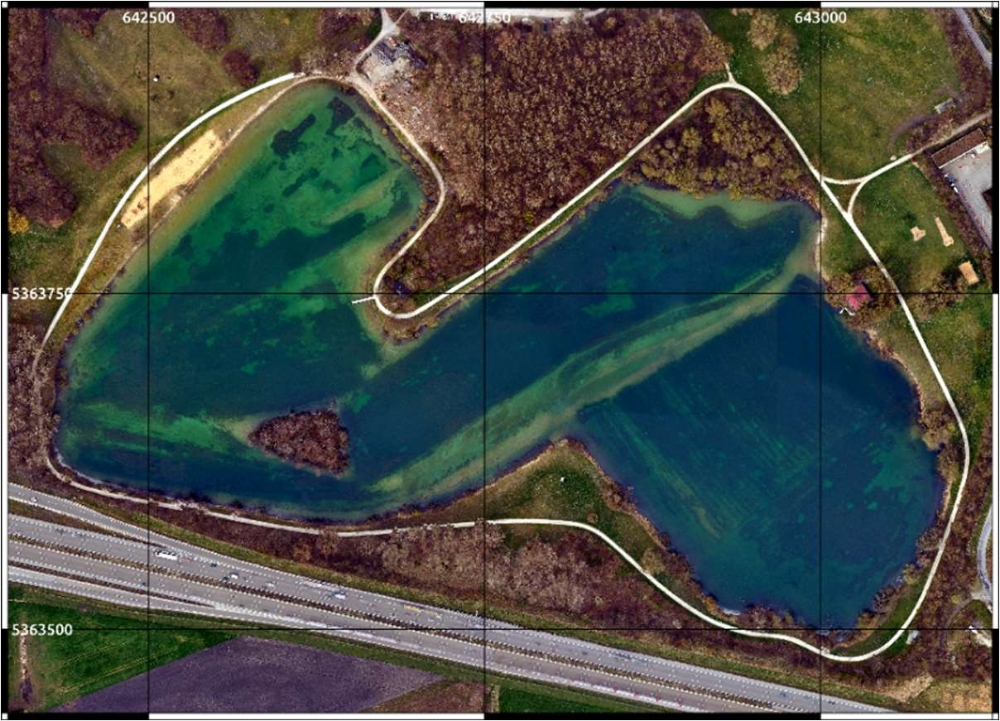
In the following, the acquisition of the investigated data is addressed. The images used for the processing were taken at the ”Autobahnsee” in Augsburg (Figure 1), which is approximately up to 5 meters deep and has a small isle as well as multiple vegetation patches and a complex elevation profile. For data acquisition two IGI DigiCAM 100 cameras are used, which are based on PhaseOne iXU-RS 1000 cameras with 11608 by 8708 pixels each, one equipped with an RGB sensor and the other with a pan-chromatic sensor and a filter for the Coastal Blue wavelength (Mandlburger et al., 2018). Using the information from both images, the same position and orientation is required. But for practical reasons the cameras had to be mounted side by side 2.2. Therefore, the Coastal Blue image is transformed into the RGB datum using a homography with the Software MATLAB (2018).

 LiDAR

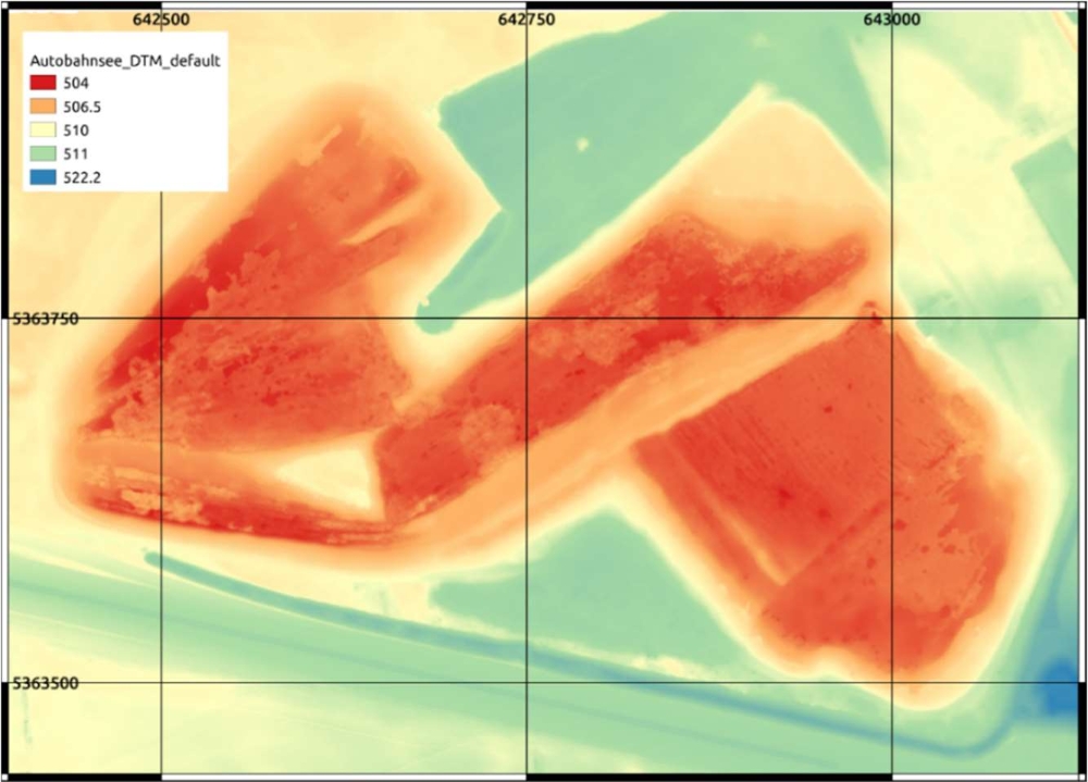
Moreover, the employed hybrid sensor system also integrates a RIEGL VQ-880- G topo- bathymetric laser scanner (Riegl, 2019) to obtain a point cloud, from which the water surface model and ground model can be extracted. In Figure 2 the ground model for the observed area is depicted. It is noted that there are complex structures at the ground of the lake caused by the distribution of soil and vegetation. These will be used to extract the reference data, being the slanted distances of the image rays in the water. The scanner is designed for shallow water mapping. Therefore, a green laser with wavelength 532 nm is used, because of its capability to penetrate water for measuring the ground of a waterbody and available high energy laser sources (Doneus et al., 2015). The mean point density of the obtained point cloud is about 40 points per square meter to get a dense model.

Preprocessing reference data

The following Section is discussing the applied methodology to derive the reference data the applied CNN is to be trained with. It is given by the respective slanted distances of the rays of every pixel in the water. To obtain them, the orientations of the camera and a water surface model (WSM), as well as a ground model are used to trace the path of rays from the camera to the corresponding ground point with consideration of refraction at the water surface. The WSM is estimated from the first echoes of the laser scanner, while the last echoes constitute the basis for filtering the ground points and, finally, calculating the Digital Terrain Model (DTM) the ground model.

In order to get the slanted distances, the rays corresponding to the individual pixels can be calculated in the local camera coordinate system using the interior orientation of the camera. They can then be transformed into a global coordinate system with help of the pixel coordinates, as well as positions and orientations of the camera at the time of exposure (Kraus and Waldhausl, 1996). Those steps are implemented in python, using the orientation file containing the interior and exterior orientations.

The next step then is to intersect the rays with the WSM, which is done using the Software OPALS (Pfeifer et al., 2014). After the intersection points of the rays with the water surface are known, for their further propagation they have to be corrected due to refraction following Snell’s law (Kotowski, 1988). That results in a change of direction for the ray depending on the incidence angle (Figure 3).

The refracted ray starting from the particular intersection point with the water surface, is afterwards intersected with the ground model, which gives the observed ground point in the respective pixel. By knowing the two intersection points, the euclidean distance can be calculated, constituting the slanted distance through the waterbody. With that information a reference raster for every image can be created. An example of that can be seen in Figure 5.1. The last step of preprocessing the data, is to mask the multispectral images, so that only pixels with valid reference depths are included.

Deep Learning

The U-Net (Ronneberger et al., 2015) serves as basis for the applied CNN. Other than in most approaches, the net is not being used for segmentation, but for fitting a regression model. So instead of having multiple classes with a normalized output for every pixel, only one quantity is trained, containing floating point numbers for the water distance of each pixel.

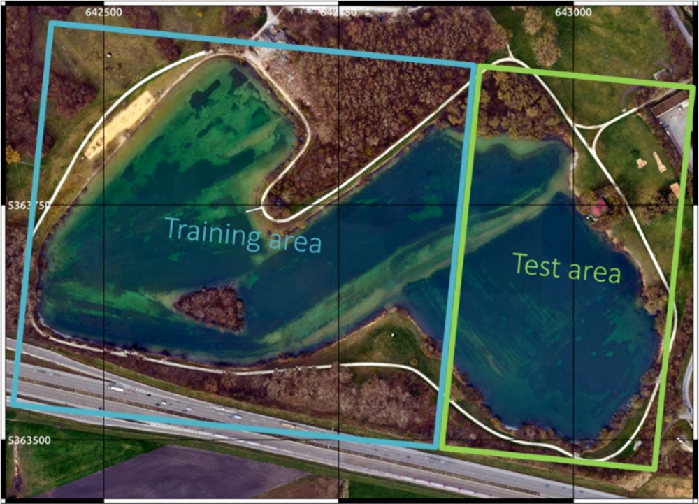
To train a net, the images have to be separated into training images, which also contain a percentage of validation data, and test images which are not used at the training. For that, the lake area is split into two parts, which are marked in Figure 4. To make sure that the test data is completely new to the net, the images containing both areas were neither used in training, nor for testing. The structures in the chosen areas differ rather strongly, so that it is possible to evaluate if the network is overfitting to the training area, or if it is learning characteristics that may be transferable also to other waterbodies.

Applied CNN for combined RGB und Coastal Blue band

Applying the trained net to previously unseen data provides an independent performance test of the net. This data consists of a subset of all images, marked as test images. Thus, it can be verified how well the net really learned certain characteristics instead of just memorizing the training data. An example for the prediction of a test image compared to the reference data can be seen in Figure 5. Despite the area on the upper right, in which the slanted underwater distances are predicted as too large, the predicted values seem to match the reference. Besides, there is no major discrepancy considering the trend of the water distances. What can be observed however, is a certain noise that may be caused by the camera sensor or by dynamics of the water surface.

After all test images are predicted, per-pixel distance deviations can be calculated by subtracting the predicted distance from the reference distance. By merging the deviations for all pixels of all test images, a histogram over all depth deviations (Figure 6) can be obtained. It is noted that only water pixels are taken into account whereas all pixels in vegetation and on dry land are masked.

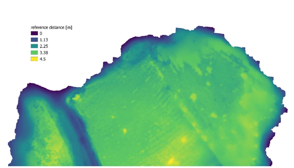
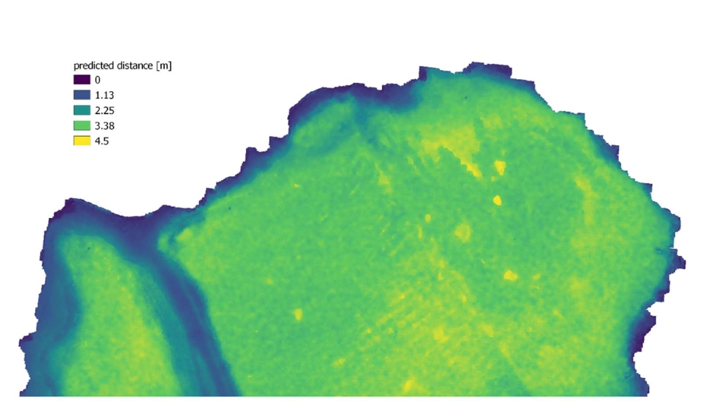
The histogram is showing an offset of one to two decimeters in negative direction, meaning that the predicted distances are larger than the reference (i.e. over estimation of water depth). It is nearly normally distributed with a median absolute deviation of 31.9 cm. The standard deviation is higher but the value is not as robust, considering outliers.

While convolution kernels are taking information from surrounding pixels into account, they tend to blur strong edges. Thus, large deviations can be found at transitions from vegetation (dark) to bare soil (bright).

Considering that the area in the test images is unknown to the model, the predictions are consistent. If the desired accuracy has to be more precise than decimeter range, the method of choice would still be SoNAR or LiDAR. If not, advantages of CNN based bathymetry estimation over the stereo photogrammetric and linear regression approach are shown in this thesis. Because of the different ground covers of the lake, a more complex model than linear regression is required.

A common issue when trying to predict features is the lack of data. The major advantage from remaining in the image system instead of projecting into a global system is shown here. It results in the possibility of using the whole dataset with all overlapping areas without reducing it. This also is the reason, why it was possible to reject the images that covered both, the training and testing area, so that there was no connection.

To see how well the net is performing for alike datasets it is reasonable to apply or transfer it to another lake or shallow waterbody. Ideally, the net can be used without any changes. Otherwise the pre-trained weights could be adapted by training with new reference under-water distances. In that case less training data should be necessary. When thinking about the advantages in terms of effort it would furthermore be interesting to see how well it performs for satellite imagery, probably after applying atmospheric corrections.

Proceeding with this method, the next logical step would be to derive a 3D point cloud from the predicted under-water distances in the images. For this purpose, an estimated water surface model and the orientations of the camera for each slanted distance image would be required. By doing  so, it is possible to analyze the overlapping areas of consecutive images, to see how well they fit. Furthermore, outliers that only occur in single images, for example because of sunglint, could be rejected by calculating the median in a certain area when creating a DTM. This could avoid the necessity of introducing further postprocessing steps.

DONEUS, M., MIHOLJEK, I., MANDLBURGER, G., DONEUS, N., VERHOEVEN, G., BRIESE, C. & PREGESBAUER, M., 2015: “Airborne laser bathymetry for documentation of submerged archaeological sites in shallow water.” In: Underwater 3D Recording and Modeling (ISPRS TC V, CIPA). Vol. 40. ISPRS, 99–107.

KOTOWSKI, R., 1988: “Phototriangulation in multi-media photogrammetry.” In: International Archives of Photogrammetry and Remote Sensing 27.B5, 324–334.

KRAUS, K. & WALDHAUSL, P., 1996: Photogrammetrie Band 2, Verfeinerte Methoden und Anwendungen. Auflage, Dümmler, Bonn.

MAAS, H.G., 2015: On the accuracy potential in underwater/multimedia photogrammetry. Sensors, 15(8), 18140-18152.

MANDLBURGER, G., KREMER, J., STEINBACHER, F. & BARAN, R., 2018: Investigating the use of Coastal Blue imagery for bathymetric mapping of inland water bodies. International Archives of the Photogrammetry, Remote Sensing & Spatial Information Sciences.

MATLAB, 2018: version 9.5.0 (R2018b). Natick, Massachusetts: The MathWorks Inc.

PFEIFER, N., MANDLBURGER, G., OTEPKA, J. & KAREL, W., 2014: OPALS–A framework for Airborne Laser Scanning data analysis. Computers, Environment and Urban Systems, 45, 125-136.

RIEGL, 2019: RIEGL VQ-880-G: Fully Integrated Topo-Hydrographic Airborne Laser Scanning System. 
http://www.riegl.com/uploads/tx_pxpriegldownloads/Infosheet_VQ-880-G_2016-05-23.pdf.

RONNEBERGER, O., FISCHER, P. & BROX, T., 2015: U-Net: Convolutional networks for biomedical image segmentation. International Conference on Medical image computing and computer- assisted intervention, Springer, 234-241.